
Plot a phylogeny in R using ggtree
Published:
This post will show you how to generate a phylogeny plot in R, with a heatmap alongside it. This example uses binary data, but it can be adapted to be plotted with a continuous variable.
First open your tree result (e.g. from IQTREE-2 or MrBayes) in FigTree, and format it there (rooting, displaying bootstrap or posterior probability values, branch swapping, etc.). Then save it as a Nexus file using the Export Trees option and select the checkboxes for Save as currently displayed and Include Annotations. The Nexus file can then be read into R using the treeio library function read.mrbayes() (even though this is an ML tree from IQTREE).
The binary data Excel file should follow a format like the one shown below. Sample names, exactly as they are in the tree file, should be in the first column. The other column names could be anything for which you have presence-absence data (e.g. presence on a particular host plant, sex, dead or alive, etc.).
| sample_ID | Arundo_donax | Cynodon_dactylon | Eragrostis_biflora | Eragrostis_capensis |
|---|---|---|---|---|
| MN133285 | 0 | 0 | 1 | 1 |
| MN133288 | 1 | 0 | 0 | 0 |
| MN133296 | 0 | 0 | 1 | 0 |
| KCP_2020_00037 | 0 | 1 | 0 | 0 |
| GFS_2020_00614 | 0 | 1 | 0 | 0 |
| GFS_2020_00562 | 0 | 0 | 1 | 1 |
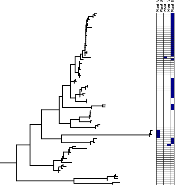
The image below is a cropped version of a phylogeny I have created using the code below.
################################
# Maximum Likelihood Phylogeny
################################

iqtree_result = treeio::read.mrbayes("C:/Users/s1000334/Documents/PhD_Tetramesa/Raw Sequences/Tetramesa/ALIGNED_READY/Tetramesa/Concatenated/Bruchophagus_removed/Singletons_removed/ML_concat_tree_R.nex")

# Have a look at the names of the features associated with the tree. Use the name given for the support values in the next bit of code (e.g boots, UFboot, bootstrap, in the case of an ML tree, or prob if it's a Bayesian tree)

iqtree_result

#change between UFboot and boots depending on how you have named this in FigTree

iqtree_iotree = iqtree_result %>% ggtree::ggtree(., color="black", layout = "rectangular", lwd=0.5) +
  geom_tiplab(size=1, color="black", font = 1) +
  geom_label2(aes(subset=!isTip, label=round(as.numeric(boots),2)), size=3, color="black", alpha=0, label.size = 0, nudge_x = -0.001) +  # add node numbers  +
  geom_treescale(fontsize=4, linesize=1)

# have a quick look at the tree

iqtree_iotree

##############################
# add host plant info
##############################

# read in an Excel file with values associated with each sequence in the phylogeny (e.g. presence-absence data)

host.plants = readxl::read_xlsx("G:/My Drive/Tetramesa Project/Source Modifiers/source_modifiers_updated_10_06_2021.xlsx",
                                sheet = "host_plants")

head(host.plants)

# change the NA cells to zeros

host.plants[is.na(host.plants)] <- 0

# change the numeric values to characters

host.plants[] <- lapply(host.plants, as.character)

# make the first column the row names

host.plants = tibble::column_to_rownames(host.plants, var = "sample_id")

# add heatmap alongside the phylogeny plotting the binary values

binary_phylo =  ggtree::gheatmap(iqtree_iotree, host.plants,
                         color="black",
                         offset=0.05, width=0.2, colnames_position = "top",
                         colnames_angle = 90, font.size=1,
                         colnames_offset_y = 2
                         ) +
  scale_fill_manual(values=c("white", "darkblue")) +
  theme(legend.position="bottom") +
  geom_treescale()

plot(binary_phylo)

# Additional plot:
# Plot the phylogeny skeleton (no tip labels)

frame = iqtree_result %>% ggtree::ggtree(., color="black", layout = "rectangular", lwd=0.5) +
  #geom_tiplab(size=1, color="black", font = 1) +
  #geom_label2(aes(subset=!isTip, label=round(as.numeric(boots),2)), size=3, color="black", alpha=0, label.size = 0, nudge_x = -0.001) +  # add node numbers  +
  geom_treescale(fontsize=4, linesize=1)

frame
